- Basics: Connecting eye tracker & EEG
- Basics: Synchronization signals
- Step 1: Convert eye tracking data to text
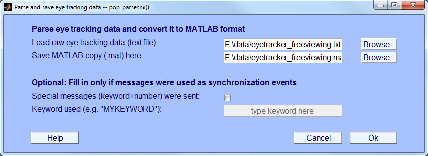
- Step 2: Preprocess eye track and store as MATLAB structure
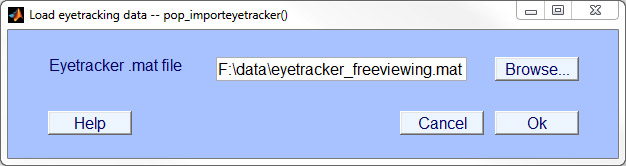
- Step 3: Load & synchronize eye track
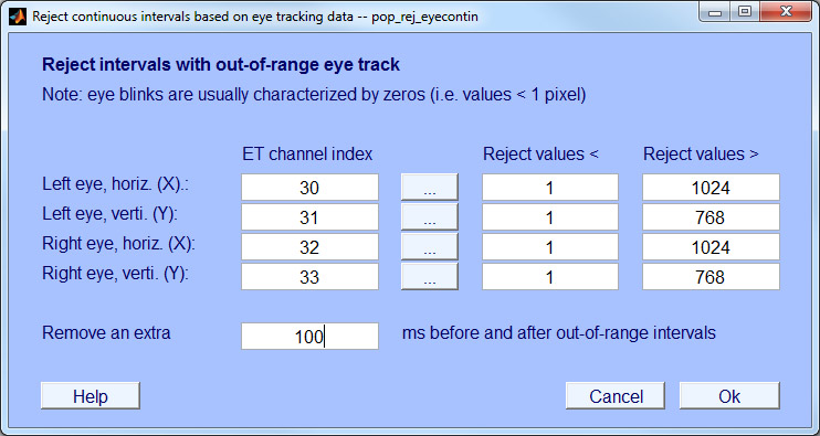
- Step 4: Reject data based on eye tracker
- Step 5: Check synchronization accuracy (via cross-correlation)
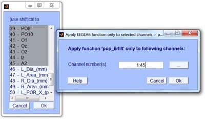
- Step 6: Apply EEGLAB function to selected channels
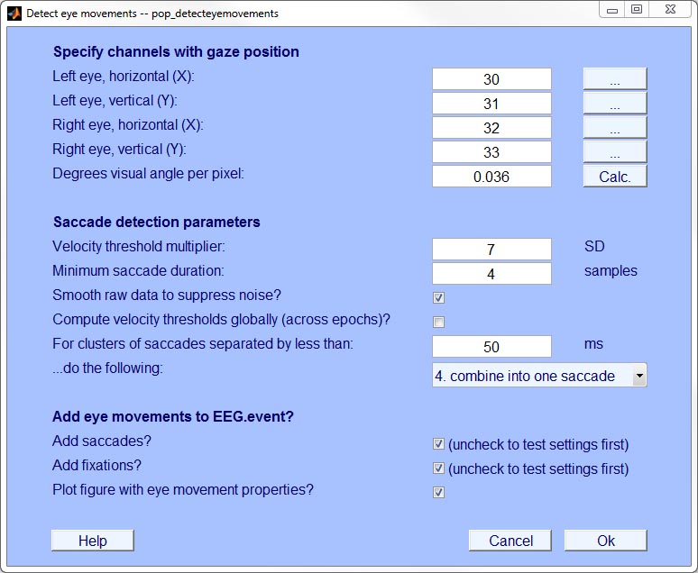
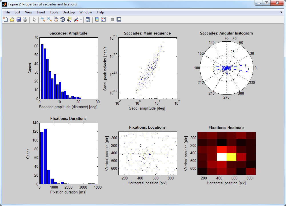
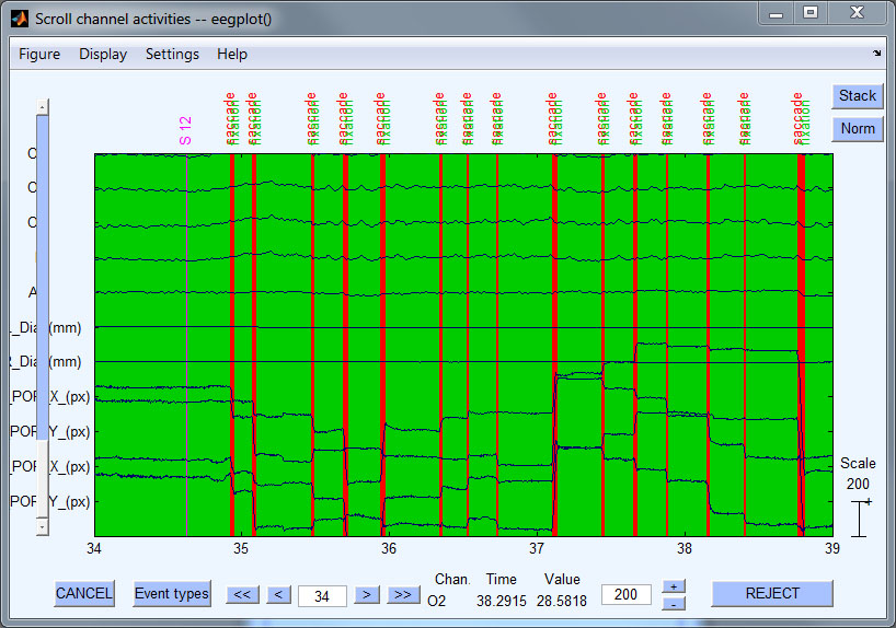
- Step 7: Detect saccades & fixations
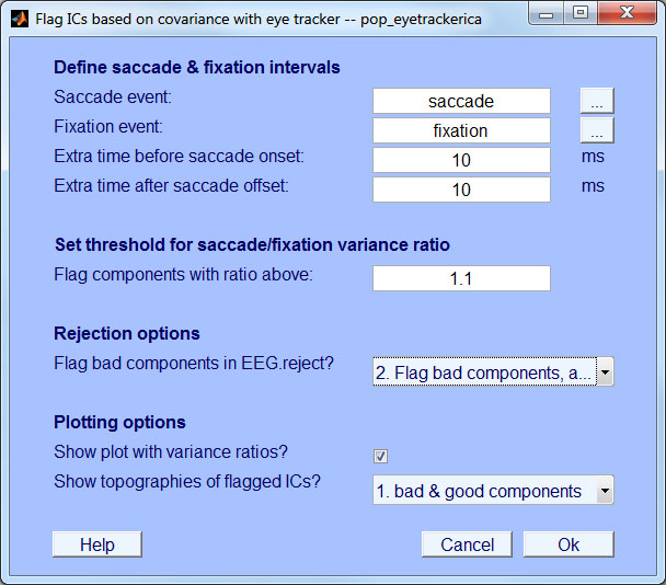
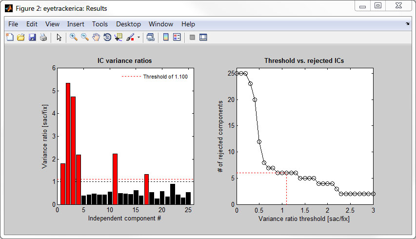
- Step 8: Remove ocular artifacts with eye tracker-guided, optimized ICA
- Writing scripts
Basics: Connecting eye tracker & EEG
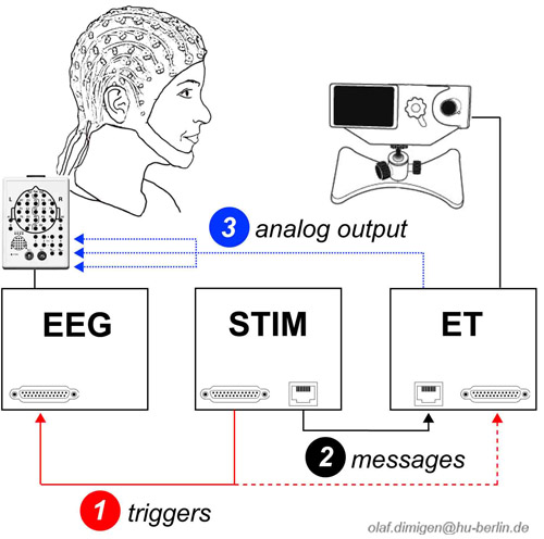
Meaningful analyses of simultaneously recorded eye tracking (ET) and EEG data requires that both data streams are synchronized with millisecond precision. There are at least three ways to synchronize both systems (Dimigen et al., 2011). The toolbox is compatible with all three, although we recommend the first one:
1: Shared triggers
Common trigger pulses ("triggers") are sent frequently from the stimulation computer to both ET computer and EEG recording computer. This is achieved via a Y-shaped cable that is attached to the parallel port of the stimulation computer and splits up the pulse so it is looped through to EEG and ET. We recommend to send triggers with a sufficient duration (e.g. at least 5 ms at 500 Hz sampling rate) to avoid the loss of some of the triggers. The advantage of this method is that the same physical signal is used for synchronization (although this does not guarantee that the trigger is inserted into the ET and EEG data streams without delays). The disadvantage is the need for an extra cable.
2: Messages+triggers
Messages are short text strings that can be inserted into the eye tracking data. While triggers are still sent to the EEG, messages are used as the corresponding events for the ET. Here, the ET computer is given a command to insert an ASCII text message (containing a keyword and the value of the corresponding EEG trigger) into the eye tracking data. In the stimulation software, the commands to send a trigger (to the EEG) and a message (to the ET) are given in immediate succession (see example code below).
3: Analogue output
A copy of the eye track is fed directly into the EEG. A digital-to-analogue converter card in the ET outputs (some of) the data as an analogue signal. With SMI, this signal can be fed directly into the EEG headbox. This requires a custom cable and resistors to scale the output voltage of the D/A converter to the EEG amplifier's recording range. While this method affords easy synchronisation, there are disadvantages: First, voltages need to be rescaled to pixels for analysis. Second, the ET signal may exceed the amplifier’s recording range and electrical interference with the EEG is possible. Third, additional information from the ET (messages, eye movements detected online) is not available. Fourth, quality of the ET signal suffers considerably from the D/A and subsequent A/D conversion. Finally, fewer channels remain to record the EEG (recording binocular gaze position and pupil diameter occupies six channels).
We recommended to test the timing accuracy of your hardware setup. For example this could mean to send triggers (and/or messages) to the eye tracker at known time intervals and to check for jitter in the recorded inter-trigger (inter-message) intervals. Also make sure to run the new ET-EOG cross-correlation test on at least a few participants (explained in Step 5 below).
Basics: Synchronization signals
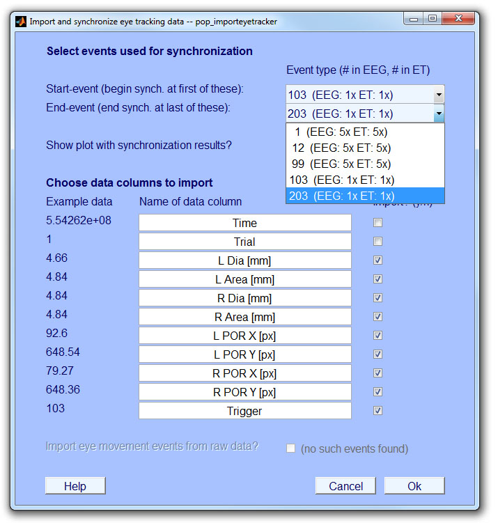
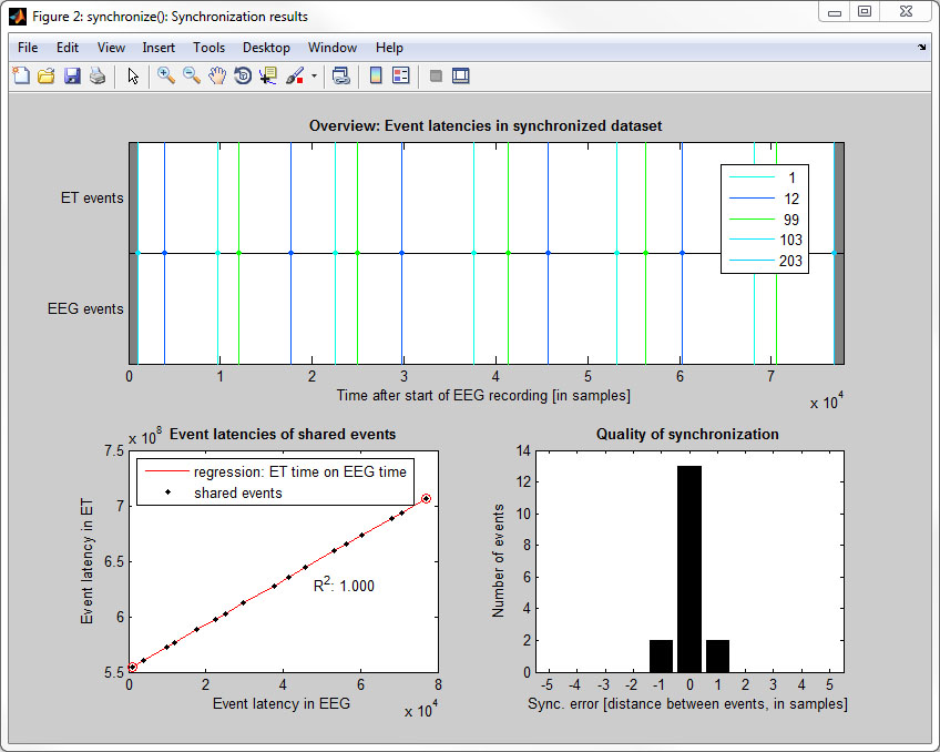
The toolbox requires that there are at least two shared events present in the ET and EEG: One near the beginning and one near the end of the recording. These events will be called start-event and end-event in the following. Eye tracking data in between the start-event and end-event will be linearly interpolated to match the sampling frequency of the EEG. We recommend to use a unique event value (e.g. "100") to mark the start-event and another unique event-value (e.g., "200") for the end-event. The remaining shared events (triggers or messages) sent during the experiment (between start-event and end-event) are used to evaluate the quality of synchronization. Synchronization is possible even if some intermediate events were lost during transmission.
Original sampling rates of EEG and ET do not need to be the same. The ET will be resampled to the sampling frequency of the EEG. For example, if the EEG was sampled at 500 Hz, and eye movements were recorded at 1000 Hz, the toolbox will downsample the eye track to 500 Hz. Since ET data outside of the synchronization range (before start-event, after end-event) cannot be interpolated, it is replaced by zeros. Please note that the EEG recording should not be paused during the experiment. [Clarification, April 2013: It is not a problem to pause the eye tracker recording, e.g. for recalibrations, because the time stamp assigned to each ET sample continues to increase even during the pause. However, the toolbox currently cannot recognize and handle pauses in the EEG recording. Therefore, the EEG recording should be continuous and must not be paused.]
Note:The current Beta version of the toolbox does not yet implement low-pass filtering of the eye track to prevent aliasing in case that the eye track is downsampled to a much lower EEG sampling rate. We plan to add this in the future.
If synchronization method 2 (messages plus trigger) is used, synchronization messages sent to the eye tracker need to have a specified format. This format consists of an arbitrary user-defined keyword (e.g., "MYKEYWORD") followed by an integer value ("MYKEYWORD 100"). The integer value needs to be the same as that of the corresponding trigger pulse sent to the EEG (usually an 8-bit number between 1 and 255). An example is given in the code below. The EYE-EEG parser (Step 2: Preprocess eye track and store as MATLAB) will recognize messages with the keyword and treat them as synchronization events. A keyword-synchronization messages should be sent together with every trigger sent to the EEG, so intermediate events in-between start-event and end-event can be used to assses synchronization quality. Additional messages (that do not contain the keyword) may be sent to code other aspects of the experimental design. They are ignored by the toolbox.
The following code is an example for an experimental runtime file containing the necessary synchronization signals. The example is for the software Presentation™, but similar commands exist in other software (e.g., Psychtoolbox, EPrime™):
# increase default duration of trigger pulses (to 6 ms)
pulse_width = 6;

# define parallel port
output_port myparallelport = output_port_manager.get_port(1);

# create eyetracker object (hex code is vendor-specific)
eye_tracker myET = new eye_tracker("{FF2F86B9-6C75-47B7-944F-2B6DECA92F48}");

myET.set_recording(true);

# beginning of experiment: send unique start trigger (or message) to ET & EEG
myparallelport.send_code(100);
myET.send_string("MYKEYWORD " + string(100)); # only needed for method 2

# [ …code of actual experiment… ]

# end of experiment: send unique end trigger (or message) to ET & EEG
myparallelport.send_code(200);
myET.send_string("MYKEYWORD " + string(200)); # only needed for method 2

myET.set_recording(false);
More information about synchronization is found in Step 3: Load and synchronize eye track.
Step 1: Convert eye tracking data to text
For use with this toolbox, the raw ET data (in binary format, *.edf or *.idf) needs to be converted to plain text (ASCII).
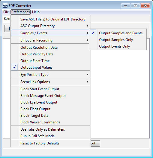
Please use the following settings in the converter software provided by the manufacturer: